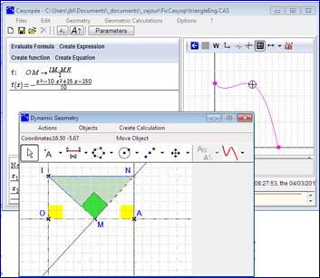
We study the dependency between two geometrical variables trough the example of the optimization of an area.
Consider the points I(0;5), O (0;0) and A (10;0). M belongs to the segment [OA], N is on the parallel to the y-axis passing by A and the triangle IMN is rectangle in M… The problem is to find the positions of M to maximize the triangle’s area.
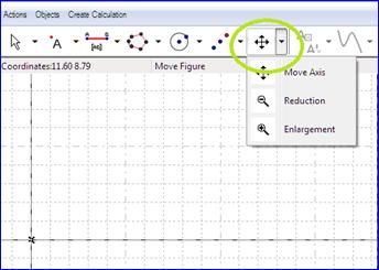
Constructing:The button interface is similar to GeoGebra’s. Each button gives access to a set of capabilities. If necessary, ask for help from somebody who knows about GeoGebra. We will first adapt the screen with the button allowing to move the screen and to zoom. |
Figure 87 -Zooming and moving axis |
|
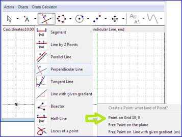
Then we create a line perpendicular to the x-axis at the point (0, 10), and then the segment from the origin to this point. Creation of segment and perpendicular are under the same button. Points are created by clicking at the appropriate place. Often several types of points are possible, and we have to choose by way of a menu. |
Figure 88 - Creating a perpendicular line and a segment |
|
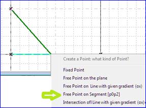
We create by the same way a segment from the point (5,0) towards a free point on the segment that has been just created. Take care to choose the adequate point in the menu. |
Figure 89 - Creating a segment towards a free point |
|
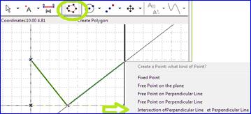
Then we create the perpendicular to the segment passing through the free point. The polygon button helps to create a triangle by clicking each point in succession and finishing by clicking again the first. The point at the intersection of the perpendicular lines has not been created before. That is why a menu opens. |
Figure 90 - Creating a triangle |
|
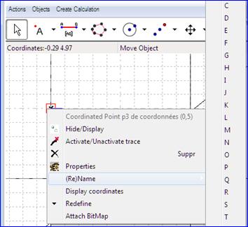
Now we name the vertexes. It is done via the (right click) contextual menu. |
Figure 91 - Naming vertexes |
|
We can also create angles by way of the button used above for polygons : one has to click on three points (I, M, N for instance) |
Figure 92 - Creating angles |
|
Here angles chosen are coded as right angles. One can display other elements (area, coordinates…) also by way of the contextual menu. |
Figure 93 - Displaying areas |
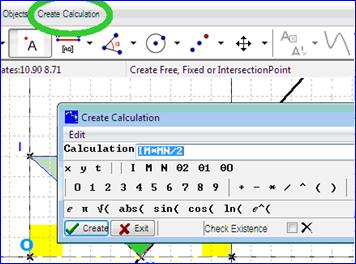
ModellingWe will now model the dependency between the position of M and the triangle area. We choose two variables: the distance OM and the formula IMxMN/2. Activating the Create calculation entry in the geometry menu, an entry box opens and we enter successively the two calculations. |
Figure 94 - Creating geometric calculations |
|
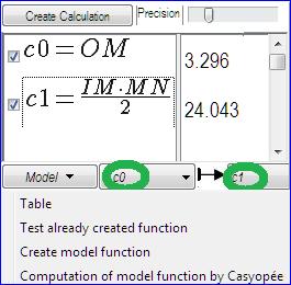
Casyopée gives two labels c0 et c1. Then we can choose them in the lists on the right of the Model button respectively as the independent and dependant variables. Numerical values of the calculations are updated when moving the free point. It helps to detect possible errors in the formulas. |
Figure 95 - The Model button |
|
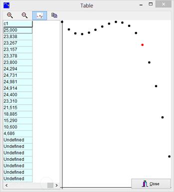
The Model button opens a menu. We choose the first entry: Table. Values taken by the two calculations for a series of positions of point M are displayed. The button The graphic visualisation on the right helps to conjecture a functional dependency from c0 to c1. In the next step we will model algebraically this dependency. |
Figure 96 - Table in the Model menu |
|
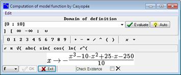
In the Model menu, we now choose the last entry: Computation of model function by Casyopée. The domain and a formula for the function are computed by Casyopée. |
Figure 97 - Computation of domain and formula by Casyopée |
|
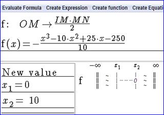
After you accept the data, the function is created in the Algebra tab. The diagram is displayed if you checked the existence. It is then easy to prove with the help of Casyopée, properties of the variations of the triangle area already conjectured by observing the figure. |
Figure 98 - Creation of a function modelling a geometric dependency |
AnimatingSwitching towards Geometry and Graph tabs, it is possible to move together the free point M on segment [OA] and the trace on the function’s graph. Here, the geometry tab has been detached by way of the Action menu. To animate the figure, assign a speed to the point M (right click menu, properties). Save the screen (main menu Files) and you will get an animated GIF. |
Figure 99 - Animating a model |
|
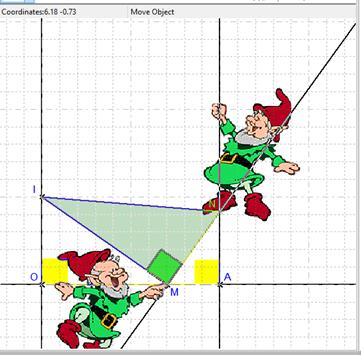
In the contextual menu of each point, the entry Attach Bitmap allows to insert a picture (bmp, jpg, or gif) that will follow the point. Like for labels, the picture can be moved relatively to the point, and resized. |
Figure 100 - Attaching pictures to points |
Note : Above, the domain of definition and the formula have been calculated by Casyopée. You may wish to compute these elements alone, either because Casyopée did not succeed or because you want to model by yourself. The entries Test already defined function and Create model function of the Model menu are there for that. The first one checks whether a function already defined in the Agebra tab can be a model. With the second entry, you create a function and it is checked like with the preceding entry. In all cases, Casyopée issues a diagnostic, either successful modelling, or an algebraic equality that Maxima could not verify. In this latter case, you have to do the verification by yourself.
 Preview
 Print...


